How To Draw 3 By 3 Gaussian Filter

Gaussian Smoothing

Mutual Names: Gaussian smoothing

Brief Description

The Gaussian smoothing operator is a ii-D convolution operator that is used to `blur' images and remove item and noise. In this sense information technology is similar to the mean filter, but it uses a different kernel that represents the shape of a Gaussian (`bell-shaped') hump. This kernel has some special properties which are detailed below.

How It Works

The Gaussian distribution in i-D has the class:

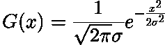
where is the standard deviation of the distribution. We have also assumed that the distribution has a mean of zero (i.e. it is centered on the line ten=0). The distribution is illustrated in Figure 1.

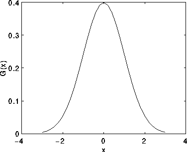
Effigy ane 1-D Gaussian distribution with mean 0 and =1

In 2-D, an isotropic (i.e. circularly symmetric) Gaussian has the form:

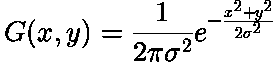
This distribution is shown in Figure 2.

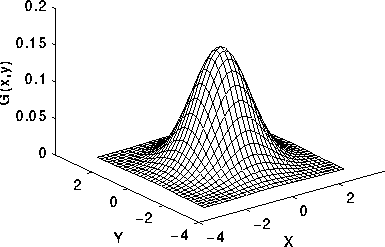
Figure 2 2-D Gaussian distribution with mean (0,0) and =1

The idea of Gaussian smoothing is to use this two-D distribution as a `indicate-spread' role, and this is achieved by convolution. Since the epitome is stored equally a collection of discrete pixels we need to produce a discrete approximation to the Gaussian office before we can perform the convolution. In theory, the Gaussian distribution is non-zero everywhere, which would crave an infinitely large convolution kernel, but in do it is effectively zero more than near three standard deviations from the hateful, and and then nosotros can truncate the kernel at this point. Figure 3 shows a suitable integer-valued convolution kernel that approximates a Gaussian with a of 1.0. It is not obvious how to pick the values of the mask to gauge a Gaussian. One could utilise the value of the Gaussian at the eye of a pixel in the mask, just this is non accurate considering the value of the Gaussian varies not-linearly across the pixel. We integrated the value of the Gaussian over the whole pixel (by summing the Gaussian at 0.001 increments). The integrals are not integers: we rescaled the array and then that the corners had the value 1. Finally, the 273 is the sum of all the values in the mask.

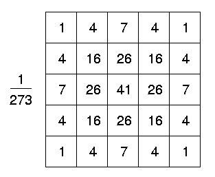
Figure three Discrete approximation to Gaussian function with =one.0

Once a suitable kernel has been calculated, and then the Gaussian smoothing can be performed using standard convolution methods. The convolution tin in fact be performed adequately quickly since the equation for the 2-D isotropic Gaussian shown above is separable into x and y components. Thus the two-D convolution tin can exist performed by start convolving with a i-D Gaussian in the x management, and and so convolving with another 1-D Gaussian in the y direction. (The Gaussian is in fact the just completely circularly symmetric operator which tin be decomposed in such a style.) Effigy 4 shows the 1-D x component kernel that would be used to produce the full kernel shown in Figure 3 (afterward scaling by 273, rounding and truncating one row of pixels around the boundary because they mostly have the value 0. This reduces the 7x7 matrix to the 5x5 shown above.). The y component is exactly the same only is oriented vertically.

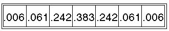
Figure 4 One of the pair of 1-D convolution kernels used to calculate the full kernel shown in Figure 3 more quickly.

A further way to compute a Gaussian smoothing with a large standard deviation is to convolve an image several times with a smaller Gaussian. While this is computationally complex, it can have applicability if the processing is carried out using a hardware pipeline.

The Gaussian filter not only has utility in engineering applications. It is also attracting attending from computational biologists because it has been attributed with some amount of biological plausibility, eastward.g. some cells in the visual pathways of the encephalon often accept an approximately Gaussian response.

Guidelines for Employ

The upshot of Gaussian smoothing is to blur an image, in a like fashion to the mean filter. The degree of smoothing is determined by the standard departure of the Gaussian. (Larger standard deviation Gaussians, of course, require larger convolution kernels in club to be accurately represented.)

The Gaussian outputs a `weighted average' of each pixel's neighborhood, with the average weighted more towards the value of the cardinal pixels. This is in contrast to the mean filter's uniformly weighted average. Because of this, a Gaussian provides gentler smoothing and preserves edges better than a similarly sized mean filter.

1 of the principle justifications for using the Gaussian as a smoothing filter is due to its frequency response. Most convolution-based smoothing filters act as lowpass frequency filters. This means that their effect is to remove loftier spatial frequency components from an image. The frequency response of a convolution filter, i.east. its effect on different spatial frequencies, can be seen by taking the Fourier transform of the filter. Figure 5 shows the frequency responses of a one-D mean filter with width five and also of a Gaussian filter with = 3.

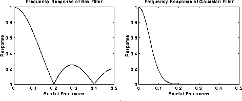
Figure five Frequency responses of Box (i.e. mean) filter (width v pixels) and Gaussian filter ( = 3 pixels). The spatial frequency axis is marked in cycles per pixel, and hence no value above 0.v has a real meaning.

Both filters benumb loftier frequencies more than than depression frequencies, just the mean filter exhibits oscillations in its frequency response. The Gaussian on the other hand shows no oscillations. In fact, the shape of the frequency response bend is itself (half a) Gaussian. And then by choosing an appropriately sized Gaussian filter we tin be fairly confident virtually what range of spatial frequencies are all the same present in the epitome later filtering, which is non the case of the mean filter. This has consequences for some border detection techniques, as mentioned in the section on aught crossings. (The Gaussian filter also turns out to be very similar to the optimal smoothing filter for edge detection under the criteria used to derive the Canny edge detector.)

We use

to illustrate the issue of smoothing with successively larger and larger Gaussian filters.

The paradigm

shows the effect of filtering with a Gaussian of = ane.0 (and kernel size 5×5).

The image

shows the effect of filtering with a Gaussian of = 2.0 (and kernel size 9×9).

The image

shows the effect of filtering with a Gaussian of = iv.0 (and kernel size 15×15).

We now consider using the Gaussian filter for noise reduction. For case, consider the paradigm

which has been corrupted by Gaussian noise with a mean of zero and = 8. Smoothing this with a 5×five Gaussian yields

(Compare this result with that achieved by the mean and median filters.)

Salt and pepper racket is more challenging for a Gaussian filter. Here we will smooth the image

which has been corrupted by one% table salt and pepper noise (i.eastward. individual bits accept been flipped with probability i%). The epitome

shows the result of Gaussian smoothing (using the same convolution as above). Compare this with the original

Discover that much of the dissonance still exists and that, although it has decreased in magnitude somewhat, information technology has been smeared out over a larger spatial region. Increasing the standard departure continues to reduce/blur the intensity of the dissonance, only also attenuates loftier frequency particular (e.g. edges) significantly, as shown in

This type of noise is better reduced using median filtering, conservative smoothing or Crimmins Speckle Removal.

Interactive Experimentation

You can interactively experiment with this operator by clicking here.

Exercises

1. Starting from the Gaussian noise (mean 0, = 13) corrupted image

   

   compute both mean filter and Gaussian filter smoothing at diverse scales, and compare each in terms of dissonance removal vs loss of detail.

2. At how many standard deviations from the mean does a Gaussian fall to 5% of its peak value? On the basis of this suggest a suitable square kernel size for a Gaussian filter with = due south.
3. Estimate the frequency response for a Gaussian filter past Gaussian smoothing an image, and taking its Fourier transform both before and later on. Compare this with the frequency response of a mean filter.
4. How does the time taken to smooth with a Gaussian filter compare with the time taken to smooth with a mean filter for a kernel of the same size? Notice that in both cases the convolution can exist speeded up considerably past exploiting sure features of the kernel.

References

East. Davies Car Vision: Theory, Algorithms and Practicalities, Academic Press, 1990, pp 42 - 44.

R. Gonzalez and R. Forest Digital Image Processing, Addison-Wesley Publishing Company, 1992, p 191.

R. Haralick and L. Shapiro Estimator and Robot Vision, Addison-Wesley Publishing Company, 1992, Vol. i, Chap. 7.

B. Horn Robot Vision, MIT Press, 1986, Chap. 8.

D. Vernon Automobile Vision, Prentice-Hall, 1991, pp 59 - 61, 214.

Local Information

Specific information nigh this operator may be found here.

More general advice about the local HIPR installation is available in the Local Information introductory section.

©2003 R. Fisher, South. Perkins, A. Walker and E. Wolfart.

Source: https://homepages.inf.ed.ac.uk/rbf/HIPR2/gsmooth.htm

Posted by: phillipsboild1989.blogspot.com

Share this post